Crisis and change have always impacted the evolution of revenue management systems (RMS). Demand shocks in the wake of global crises and evolutions in airline business models have inspired new science to optimize airline revenues.
Yet, the COVID-19 pandemic represents a unique challenge for RMS. Months of cancelled flights have left holes in RMS’ historical database, while customer booking and cancellation patterns along with their willingness-to-pay have abruptly and significantly changed from pre-pandemic levels. With such drastic changes, it may appear that the RMS demand forecaster would need to essentially start from a blank slate.
Fortunately, the reality is not so dire. Amadeus’ demand forecast already uses live sales data from non-departed flights, and as such would adjust the demand levels automatically as airlines resume operations. However, we found that in the current situation, which holds significant uncertainty about future customer demand, airlines need a forecast that can capture the most up-to-date demand patterns based on as little as a few months’ worth of live sales data.
To overcome this challenge, our revenue management research team have developed a novel demand forecast that we call Active Forecast Adjustment (AFA), which can quickly adapt to changes in market demand.
What have we done to adapt airline revenue management forecasts?
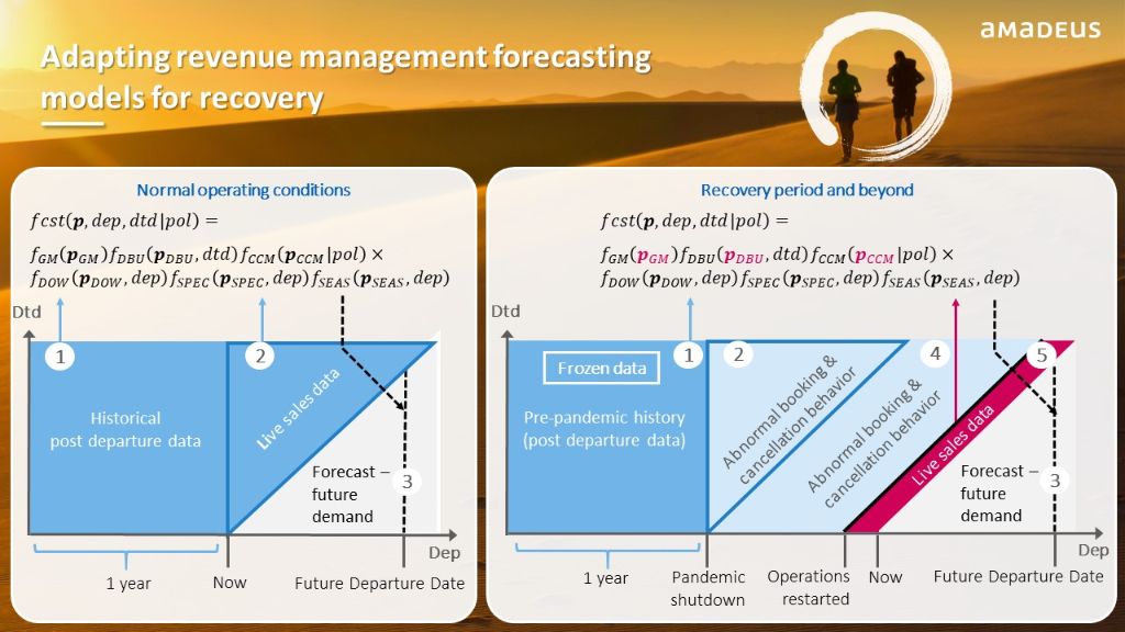
To explain the principles behind this forecast, we need to dig a little deeper into the forecasting process as represented in the graphic below. The left panel shows the RMS forecaster under normal operating conditions and the right panel shows the forecaster during the pandemic recovery period and the new normal conditions.

Since demand forecasts are needed for each future departure date and day-to-departure (light grey triangle 3), RMS typically record historical data along the same dimensions. Each day, live sales data is recorded for all future departure dates. This data is stored in the historical database, the so-called “Guillotine”, which consists of two parts: one year’s post-departure data (blue square 1) and one year’s live sales data (blue triangle 2).
The demand forecast is computed from the post-departure data (1) to allow a simultaneous estimation of all forecast components. Secondly, live sales data (2) are used to adjust forecast volumes to account for demand fluctuations of individual departure dates. Under normal operations, this approach works extremely well.
However, the pandemic shutdown has led to months of abnormal booking and cancellation behavior, threatening to pollute the historical database. To retain control, we froze the post-departure history to ensure a stable forecast based on the pre-pandemic data (1). This approach has allowed revenue management analysts to control their flights using interventions, as explained in the recent blog post “The big reset: four phases to airline revenue management strategy planning ” bySuraj Mohamed.
Widespread demand changes, such as the pandemic recovery, affect all departure dates simultaneously and will be clearly visible in the most recent live sales data. The principle behind AFA is therefore to create a feedback loop where the forecast error (actual bookings – expected bookings) on the live sales data is constantly monitored and adjustments are applied to minimize forecast errors. Unlike the previous use of live sales data (2) to fine-tune the demand for individual departure dates, AFA automatically adjusts forecasts across all departure dates based on the latest market level live sales data (5).
What is new about Active Forecast Adjustment in airline revenue management?
While using live sales data to adjust the demand forecast may seem like an obvious idea, the issue is that some forecast components (such as seasonal patterns) require extended data spanning (at least) a full year of observations. Furthermore, the amount of live sales data in the parallelogram (5) is only a fraction of the entire historical database (1+2) and is insufficient to estimate the entire forecast model.
The novelty of AFA is that it separates the components of the demand forecast into two categories, depending on if they are likely to be resilient or volatile during the recovery period. For example, we expect seasonal demand variation and day-of-week demand patterns to be largely resilient, while total demand volume, booking curves, and customer willingness-to-pay are expected to be volatile. Targeting only the volatile components with AFA enables us to reduce the complexity, so it becomes possible to adjust these components using the most recent sales data to maximize forecast accuracy.
Our initial research indicates that the principles of AFA hold considerable value beyond the pandemic recovery period. Even after we have collected enough unpolluted data to “unfreeze” the estimation of forecast parameters, AFA can still be used to ensure rapid reaction to market changes, increasing forecast adaptivity while retaining robustness and stability. As our article,Can demand forecast accuracy be linked to airline revenue? indicated, even a 10% increase in forecast accuracy can lead to a 1% gain in revenue, so AFA holds significant revenue potential for airlines.
Times of crisis often serve as a catalyst for innovation and change, and this pandemic is no exception. Our R&D and Professional Services teams are working together at full speed to make AFA available for our customers this year. This work continues together with ourMachine Learning Services team to define new data-driven models for identifying changes in demand patterns. Our goal is to have a revenue management solution that supports our airline customers through thefour phases of recovery and beyond.
TO TOP


